Problem 7.13#
The initial and boundary conditions stated in the question do not produce the analytical solution stated. Instead we will consider a slightly different system. For the domain \(x\in[0, 1]\) and boundary conditions
let us consider a different initial condition.
This system has the analytical solution
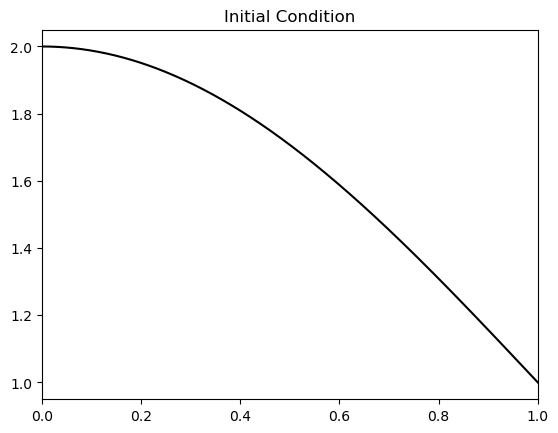
which we will model instead. Let us first plot this new initial condition
Show code cell source
import numpy as np
import matplotlib.pyplot as plt

# Initial condition
fig, ax = plt.subplots()
xplt = np.linspace(0, 1, 1000)
ax.plot(xplt, 1 + np.cos(0.5* np.pi * xplt), 'k');
ax.set_title('Initial Condition');
ax.set_xlim([0,1]);
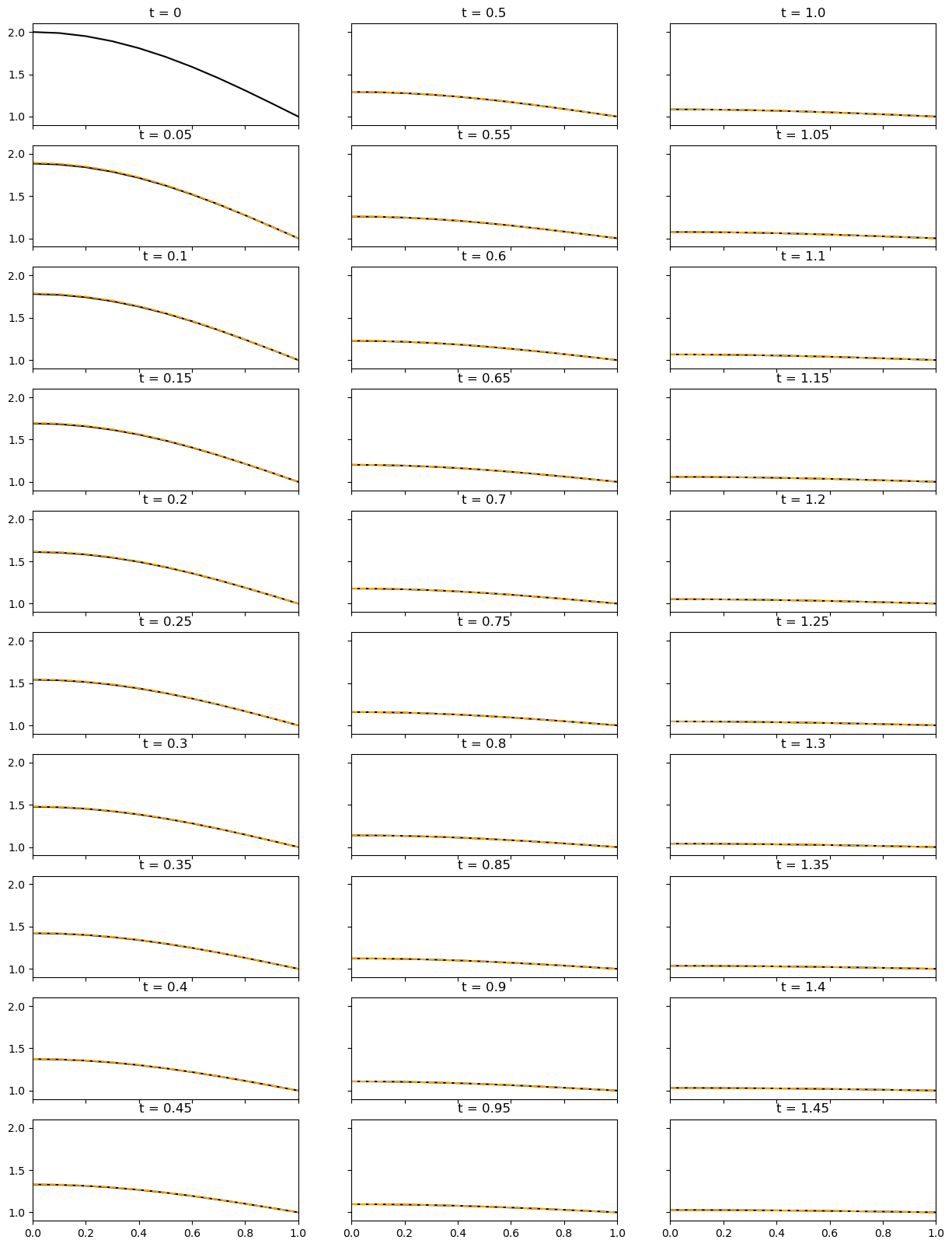
Physically, this system allows for no heat flux at the left boundary, while the RHS boundary must maintain a constant temperature. The domain has no input of heat. To facilitate these conditions, the heat must exit though the right boundary of the system, for which the heat flux is not fixed. Hence, we expect to see a decay in temperature through time until the system is at steady state.
Domain setup#
Let us define our domain numerically with 10 elements, leading to 11 global nodes.
L       = 1         # domain size
nelem   = 10        # number of elements, n
npts    = nelem + 1 # n+1

# Global domain node locations
x = np.linspace(0, L, npts)

# Compute Delta x for each element:
dx = x[1:] - x[:-1]

# Boundary conditions:
theta_1 = 1
H0      = 0
K matrix#
Next, we compute our global diffusivity matrix based on Eqns. 7.49 - 7.51
# Generate K
K = np.zeros((nelem, nelem))

for ielem in range(nelem):

    if ielem == 0:
        K[ielem, ielem] = 1 / dx[0]
    else:
        K[ielem, ielem] = (1 / dx[ielem - 1]) + (1 / dx[ielem])
        K[ielem - 1, ielem] = -1 / dx[ielem - 1]
        K[ielem, ielem - 1] = -1 / dx[ielem - 1]
Mass matrix#
The mass matrix can be similarly computed based on Eqns 7.88 - 7.90
M = np.zeros((nelem, nelem))

for ielem in range(nelem):
    if ielem == 0:
        # 7.88
        M[ielem, ielem] = dx[0] / 3
    else:
        # 7.90
        M[ielem, ielem] = (dx[ielem - 1] + dx[ielem]) / 3
        # 7.89
        M[ielem - 1, ielem] = dx[ielem - 1] / 6
        M[ielem, ielem - 1] = dx[ielem - 1] / 6
Forcing#
The force vector is given in Eqn. 7.87 as
For our case, \(h=0\) and \(H_0 = 0\) such that the force is only
at the \(n\)th node only.
F = np.zeros(nelem)
F[-1] = theta_1/(dx[-1])
Timestepping#
Finally, we can step our system of equations in time using the Generalised Trapezoidal Time Scheme discussed in Section 7.3.3. For \(\eta = 0.5\) this is a centered finite difference method in time.
eta    = 0.5    # time-scheme parameter
dt     = 0.01   # timestep
nsteps = 150    # number of timesteps

# Initialise temperature and derivative
temp       = np.zeros(npts)
dtemp_dt   = np.zeros(npts)

# Set initial condition
temp       = 1 + np.cos(0.5* np.pi * x)

# Inverse of [M + eta \delta t K]
# rearranged version of Eqn 7.92
MKinv = np.linalg.inv(M + eta*dt*K)

# Create plots of time evolution
fig, ax = plt.subplots(10, 3,
                       sharey=True,
                       figsize=(15,20),
                       sharex=True)

# Step in time
time = 0

# Plot initial condition
ax[0,0].set_title(f"t = 0");
ax[0,0].plot(x, temp, 'k')

iax = 1
icol = 0
for istep in range(1,nsteps):
    # Compute time
    time += dt

    # --- FEM calculation ---
    # Predictor:
    dtilde = temp[:-1] + (1-eta)* dt * dtemp_dt[:-1]

    # Solve for dtemp_dt at next timestep
    dtemp_dt[:-1] = np.matmul(MKinv, F - np.matmul(K, dtilde))

    # Corrector:
    temp[:-1] = dtilde + (eta * dt * dtemp_dt[:-1])

    # Plot every 5 timesteps
    if istep%5 == 0:

        # Compute analytical solution and plot
        analytical =  1 + (np.exp(- 0.25 * time * np.pi**2 ) *
                           np.cos(0.5*np.pi *x))
        ax[iax, icol].plot(x, analytical, 'k')

        # Plot FEM
        ax[iax, icol].set_title(f"t = {np.around(time,2)}");
        ax[iax, icol].plot(x, temp, 'orange', linestyle='--')

        iax += 1
        if iax==10:
            icol += 1
            iax = 0

# Some plot formatting
ax[0,0].set_xlim([0,1]);
ax[0,0].set_ylim([0.9,2.1]);