Problem 7.2#
Here we compare the solutions in Eqn 7.19 and 7.36 for the case that \(h=1\) across the domain. Starting with Eqn. 7.19
\[\begin{equation*}
\theta(x) = \theta_1 + (1-x) H_0 + \int_x^1 \int_0^y h(z) \: \mathrm{d}z \: \mathrm{d}y
\end{equation*}\]
which, for \(h(z)=1\) becomes
\[\begin{equation*}
\theta(x) = \theta_1 + (1-x) H_0 + \frac{1}{2}(1-x^2)
\end{equation*}\]
For Eqn 7.36, the solution
\[\begin{equation*}
\theta(x) = \theta_1 + (1-x) H_0 + \left[ \int_0^1 (1-y) \: \mathrm{d}y \right] (1-x)
\end{equation*}\]
becomes
\[\begin{equation*}
\theta(x) = \theta_1 + (1-x) H_0 + \frac{1}{2}(1-x)
\end{equation*}\]
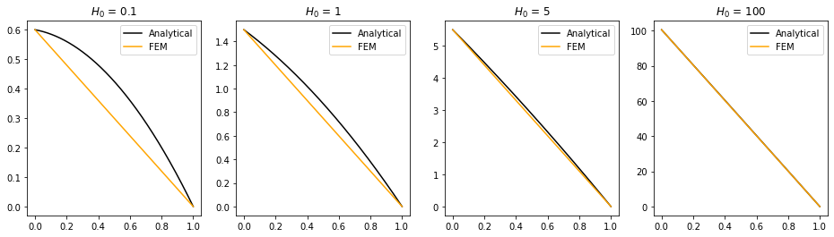
As shown below, the FEM solution is therefore acceptable when \(H_0\) is sufficiently large that the quadratic term in the analytical solution is relatively negligible, but a poor approximation otherwise.
Show code cell source
import numpy as np
import matplotlib.pyplot as plt

fig, ax = plt.subplots(1, 4, figsize=(16,4))

theta_1 = 0

H0s = [0.1, 1, 5, 100]

x = np.linspace(0, 1, 1000)
for i in range(4):

    H0 = H0s[i]
    analytical = theta_1 + (1-x)*H0 + 0.5*(1-x**2)
    FEM        = theta_1 + (1-x)*H0 + 0.5*(1-x)

    ax[i].plot(x, analytical, 'k', label='Analytical')
    ax[i].plot(x, FEM, 'orange', label='FEM')
    ax[i].set_title(fr"$H_0$ = {H0}")
    ax[i].legend()