Problem 6.8

Starting with our equation (6.75) for the grid phase speed

\[\begin{equation*} c^{\text{grid}} = \frac{2}{k\,\Delta t} \arcsin \left\{ c\,\Delta t \:\left[ \left( \frac{\sin\left( \frac{1}{2}k_x\,\Delta x \right)}{\Delta x}\right)^2 + \left( \frac{\sin\left( \frac{1}{2}k_y\,\Delta y \right)}{\Delta y}\right)^2 \right]^{1/2} \right\} \end{equation*}\]

This is written slightly differently to the textbook, collecting the powers of 2 on the sine functions and \(\Delta x\)/\(\Delta y\) outside of a bracket. Hopefully this makes it clearer for the next step of our solution.

The fact that the question tells us to use \( k_x^2 + k_y^2 = k^2 \) hints we should aim to extract the \(k_x\) and \(k_y\) from the sine functions. In fact, when \(\Delta x\) and \(\Delta y\) are small, and the argument of the sine functions tends to 0. The small-angle approximation states that as \(\theta \rightarrow 0 \) the sine function

\[\begin{equation*} \sin(\theta) \rightarrow \theta \end{equation*}\]

Therefore since \(\Delta x \rightarrow 0\) and \(\Delta y \rightarrow 0\) we may approximate

\[\begin{align*} \sin\left( \frac{1}{2}k_x\,\Delta x \right) &\rightarrow \frac{1}{2} k_x \, \Delta x \\ \sin\left( \frac{1}{2}k_y\,\Delta y \right) &\rightarrow \frac{1}{2} k_y \, \Delta y \end{align*}\]

The equation for the grid speed then becomes

\[\begin{equation*} c^{\text{grid}} = \frac{2}{k\,\Delta t} \arcsin \left\{ c\,\Delta t \:\left[ \left( \frac{\frac{1}{2}k_x\,\Delta x}{\Delta x}\right)^2 + \left( \frac{\frac{1}{2}k_y\,\Delta y}{\Delta y}\right)^2 \right]^{1/2} \right\} \end{equation*}\]

which may be reduced to

\[\begin{equation*} c^{\text{grid}} = \frac{2}{k\,\Delta t} \arcsin \left\{ c\,\Delta t \:\left[ \frac{1}{4} \left( k_x^2 + k_y^2 \right) \right]^{1/2} \right\} \end{equation*}\]

Next, we utilise the aforementioned information that \(k_x^2 + k_y^2 = k^2\) such that this simplifies to

\[\begin{equation*} c^{\text{grid}} = \frac{2}{k\,\Delta t} \arcsin \left\{ \frac{1}{2} c\,\Delta t \: k \right\} \end{equation*}\]

Finally, dealing we must navigate the limit of the \(\arcsin\) as \(\Delta t \rightarrow 0\). A Taylor expansion of \(\arcsin(\Delta t)\) about 0 is

\[\begin{equation*} \Delta t + \frac{1}{6}(\Delta t)^3 + \mathcal{O}(\Delta t^5) \quad. \end{equation*}\]

Hence to first order we may approximate the arcsin function in this limit as simply its argument, making the speed as

\[\begin{equation*} c^{\text{grid}} = \frac{1}{2} c\,\Delta t \: k \frac{2}{k\,\Delta t} = c \end{equation*}\]

as required.

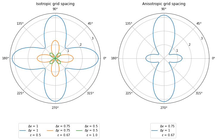
How wrong is the grid speed?

The phase speed on the grid is, as above,

\[\begin{equation*} c^{\text{grid}} = \frac{2}{k\,\Delta t} \arcsin \left\{ c\,\Delta t \:\left[ \left( \frac{\sin\left( \frac{1}{2}k_x\,\Delta x \right)}{\Delta x}\right)^2 + \left( \frac{\sin\left( \frac{1}{2}k_y\,\Delta y \right)}{\Delta y}\right)^2 \right]^{1/2} \right\} . \end{equation*}\]

Below, we plot the error between the true speed and the grid speed. These plots are inspired by Fig 4.14 of Heiner Igel’s Computational Seismology book.

import numpy as np 
import matplotlib.pyplot as plt 


k  = 1                        # Wavenumber
DX = [1, 0.75, 0.5,  0.75]    # Grid spacing in x
DY = [1, 0.75, 0.5,  1]       # Grid spacing in y
dt = 0.5                      # Timestep
c  = 1                        # True wavespeed 

# courant number for each case
courant_x = c*dt/np.array(DX);
courant_y = c*dt/np.array(DY);

# number of scenarios
nscenarios = len(DX)

# create angle over which to evaluate
# x and y given by cos and sin of theta
theta = np.linspace(0, 2*np.pi, 100)

fig, axes = plt.subplots(1, 2, figsize=(12,6), subplot_kw={'projection': 'polar'})

leglabels = []

for i in range(nscenarios): 
    
    if i < nscenarios-1: 
        ax = axes[0]
        ax.set_title("Isotropic grid spacing", va='bottom')
        bbox = (1, -0.2)

    else:
        ax = axes[1]
        ax.set_title("Anisotropic grid spacing", va='bottom')
        bbox = (0.65, -0.2)

    dx = DX[i]
    dy = DY[i]
    
    # Compute grid speed at each theta
    cgrid = (2/(k*dt)) * np.arcsin( c*dt * ((np.sin(k*np.cos(theta) * dx/2)/dx)**2 +   
                                            (np.sin(k*np.sin(theta) * dy/2)/dy)**2)**0.5)

    # Compute percentage error from 'true' c
    deltac  = 100*np.abs((cgrid - c))/c 
    
    ax.plot(theta, deltac)
    ax.set_rlabel_position(27)  # Move radial labels away from plotted line
    ax.set_rticks([1, 2, 3])    # Less radial ticks

    leglabels.append(r'$\Delta x$ = ' +f'{dx}\n' + r'$\Delta y$ = '+f'{dy}\n' 
                     + r'  $\epsilon$ = '+f'{np.around(courant_x[i],2)}')
    
    if i >= nscenarios-2: 
        ax.legend(leglabels, ncols=3, bbox_to_anchor=bbox)
        leglabels = []