Problem 7.5

The domain contains \(n+1\) nodes. However, final node (\(n+1\)) has its temperature fixed at \(\theta_1\) due to the boundary condition. As such, we do not need to ever solve for the temperature at this point.

Diffusivity matrix

The diffusivity matrix, \(\mathbf{K}\), is therefore \((n \times n)\) and for constant grid spacing \(\Delta x\) has the following components:

\[\begin{align*} K_{1\,1} &= 1/\Delta x \\ K_{A\,A} &= 1/\Delta x_{A-1} + 1/\Delta x_{A} \\ &= 2 / \Delta x \\ K_{A-1\,A} = K_{A\,A-1} &= - 1/\Delta x_{A-1} \\ &= -1 / \Delta x \\ \end{align*}\]

or in matrix format

\[\begin{equation*} \mathbf{K} = \frac{1}{\Delta x} \begin{bmatrix} 1 & -1 & & & \\ -1 & 2 & -1 & & \\ & -1 & 2 & -1 & \\ & & \ddots & \ddots & \ddots& \\ & & & -1 & 2 & -1 \\ & & & &-1 & 2 & -1 \\ & & & & & -1 & 2 \\ \end{bmatrix} \end{equation*}\]

Forcing matrix

The forcing matrix components are defined as follows:

Point \(x_1\)

\[\begin{equation*} F_1 = \frac{1}{\Delta x_1} \int_{x_1}^{x_2} (x_2 - x) \, h(x) \, \mathrm{d}x + H_0 \end{equation*}\]

in the case that \(h=0\) this is simply

\[\begin{equation*} F_1 = H_0\quad. \end{equation*}\]

In the case that \(h = 1\) this is

\[\begin{align*} F_1 &= \frac{1}{\Delta x_1} \int_{x_1}^{x_2} (x_2 - x) \, \mathrm{d}x + H_0 \\ &= \frac{1}{2 \Delta x_1} (x_2 - x_1)^2 + H_0 \\ &= \frac{1}{2} (x_2 - x_1) + H_0 \\ &= \frac{1}{2} \Delta x_1 + H_0 \end{align*}\]

Internal points (A = 2, … n)

For all points except the last (\(2, ... n-1\)), the forcing is given by

\[\begin{equation*} F_A = \frac{1}{\Delta x_{A-1} } \int_{x_{A-1}}^{x_A} (x - x_{A-1})\, h(x)\, \mathrm{d}x \:+\: \frac{1}{\Delta x_{A} } \int_{x_{A}}^{x_{A+1}} (x_{A+1} - x)\, h(x)\, \mathrm{d}x \end{equation*}\]

When \(h=0\) this produces \(F_A = 0\). When \(h=1\) this produces

\[\begin{align*} F_1 &= \frac{1}{2 \Delta x_{A-1}} \left( x_A - x_{A-1} \right)^2 + \frac{1}{2 \Delta x_A} \left( x_{A+1} - x_{A} \right)^2 \\ &= \frac{1}{2} \Delta x_{A-1} + \frac{1}{2} \Delta x_{A} \\ \end{align*}\]

which for a constant \(\Delta x\) is simply equal to \(\Delta x\) .

The \(n\)’th node contains contributions from the last element and \(\theta_1\), given in 7.54 as

\[\begin{equation*} F_n = \frac{1}{\Delta x_{n-1}} \int_{x_{n-1}}^{x_n} (x - x_{n-1})\, h(x) \: \mathrm{d}x + \frac{1}{\Delta x_{n}} \int_{x_{n}}^{x_{n+1}} (x_{n+1} - x)\, h(x) \: \mathrm{d}x \: + \frac{\theta_1}{\Delta x_n} \quad. \end{equation*}\]

For the case that \(h=0\) this reduces to

\[\begin{equation*} F_n = \frac{\theta_1}{\Delta x_n}, \end{equation*}\]

where as for \(h(x) = 1\) it is

\[\begin{equation*} F_n = \frac{\Delta x_{n-1}}{2} + \frac{\Delta x_{n}}{2} + \frac{\theta_1}{\Delta x_n}, \end{equation*}\]

Case 1: h = 0

For 10 elements (\(n=10\)) the equations then becomes

\[\begin{equation*} \frac{1}{\Delta x} \begin{bmatrix} 1 & -1 & & & & & & & & \\ -1 & 2 & -1 & & & & & & & \\ & -1 & 2 & -1 & & & & & & \\ & & -1 & 2 & -1 & & & & & \\ & & & -1 & 2 & -1 & & & & \\ & & & & -1 & 2 & -1 & & & \\ & & & & & -1 & 2 & -1 & & \\ & & & & & & -1 & 2 & -1 & & \\ & & & & & & & -1 & 2 & -1 & \\ & & & & & & & & -1 & 2 & -1 \\ \end{bmatrix} \mathbf{\Theta} = \begin{bmatrix} H_0 \\ 0 \\ 0 \\ 0 \\ 0 \\ 0 \\ 0 \\ 0 \\ 0 \\ \frac{\theta_1}{\Delta x} \end{bmatrix} \end{equation*}\]

since \(H_0\) = 1

The solution is then:

import numpy as np 
import matplotlib.pyplot as plt 

L = 1     # Domain 0 to L
n = 10    # Number of elements

# Boundary conditions
theta_1 = 1 
H0      = 1 

x = np.linspace(0, L, n+1)

dx = x[1:] - x[:-1]  # Delta x in each element

# Create matrix K
diag     =  2 * np.ones(n)     # Main diagonal
off_diag = -1 * np.ones(n-1)  # Off-diagonals
K = np.diag(diag) + np.diag(off_diag, k=1) + np.diag(off_diag, k=-1)

# Edit the first diagonal element
K[0,0]   = 1  

# Remember division by dx for K matrix
K = K/dx

# Create vector f: 

F = np.zeros(n)
F[0] = H0
F[-1] = theta_1 / dx[-1]


# Compute inverse matrix K^-1 
Kinv = np.linalg.inv(K)

# Compute theta 
theta = np.matmul(Kinv, F)

# Theta array for whole domain contains the n+1 point also: 
total_theta = np.zeros(n+1)
total_theta[:n] = theta
total_theta[-1] = theta_1



# Plot for comparison
fig, ax = plt.subplots()

# Plot FEM 
ax.plot(x, total_theta, 'k')

# Plot analytical
analytical = 1 + (1-x)*H0
ax.plot(x, analytical, '--', color='orange')
ax.legend(['FEM', 'Analytical']);

Case 2: h = 0

Now lets look at the case when \(h = 1\). Remember that \(h\) doesn’t affect the diffusivity matrix so all we need to do is compute the new \(\mathbf{F}\) vector

# Create a new F vector 
F = np.zeros(n)

for inode in range(n): 
    if inode == 0: 
        F[inode] = H0 + dx[0]/2  
    else: 
        F[inode] = 0.5 * (dx[inode-1] + dx[inode])

        
    # The last node (n) also gets an extra contribution 
    # note the python indexing from 0 here means its 'n-1'
    if inode == n-1: 
        F[inode] += theta_1/dx[inode]
        

# Now we can compute the temperature field: 
# Compute theta 
theta = np.matmul(Kinv, F)

# Theta array for whole domain contains the n+1 point also: 
total_theta = np.zeros(n+1)
total_theta[:n] = theta
total_theta[-1] = theta_1

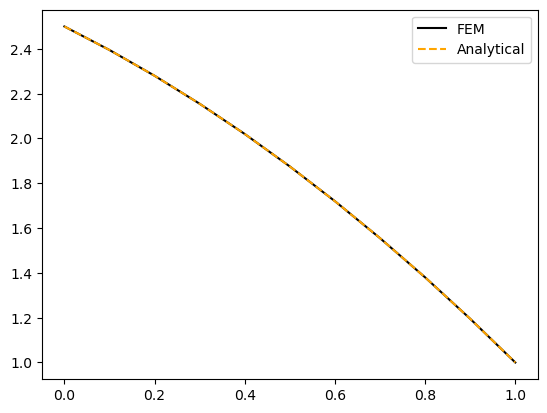
Let us compare against an analytical solution (7.19) for \(h(x)=1\) which ends up being

\[\begin{equation*} \theta(x) = \theta_1 + (1-x) H_0 + \frac{1}{2}(1-x^2) \quad. \end{equation*}\]

Note how the internal heating contributes an extra quadratic term compared to the case when \(h=0\).

# Plot for comparison
fig, ax = plt.subplots()

# Plot FEM 
ax.plot(x, total_theta, 'k')

# Plot analytical
analytical = theta_1 + (1-x)*H0 + 0.5*(1 - x**2)
ax.plot(x, analytical, '--', color='orange')
ax.legend(['FEM', 'Analytical']);