Problem 6.11
Let us take Eqn. 6.92
\[\begin{equation*}
- \frac{\gamma}{2} \theta^n_{j-1} + \left[ 1 + \gamma \right]\, \theta^n_j - \frac{\gamma}{2} \theta^{n}_{j+1} = \frac{\gamma}{2} \theta^{n-1}_{j-1} + \left[ 1 - \gamma \right] \theta^{n-1}_j + \frac{\gamma}{2} \theta^{n-1}_{j+1}
\end{equation*}\]
where \(\gamma = \frac{\alpha \Delta t}{(\Delta x)^2}\). Next as instructed we will sub in our plane wave approximations from 6.83 for the current timestep
\[\begin{align*}
\theta^{\,n}_{j-1} &= A^n \, e^{i k (j-1) \Delta x}\\
\theta^{\,n}_j &= A^n \, e^{i k j \Delta x}\\
\theta^{\,n}_{j+1} &= A^n \, e^{i k (j+1) \Delta x}\\
\end{align*}\]
and previous timestep
\[\begin{align*}
\theta^{\,n-1}_{j-1} &= A^{n-1} \, e^{i k (j-1) \Delta x}\\
\theta^{\,n-1}_j &= A^{n-1} \, e^{i k j \Delta x}\\
\theta^{\,n-1}_{j+1} &= A^{n-1} \, e^{i k (j+1) \Delta x}\\
\end{align*}\]
which yields
\[\begin{align*}
- &\frac{\gamma}{2} A^n \, e^{i k (j-1) \Delta x} + \left[ 1 + \gamma \right]\, A^n \, e^{i k j \Delta x} - \frac{\gamma}{2} A^n \, e^{i k (j+1) \Delta x} \\
= &\frac{\gamma}{2} A^{n-1} \, e^{i k (j-1) \Delta x} + \left[ 1 - \gamma \right] A^{n-1} \, e^{i k j \Delta x} + \frac{\gamma}{2} A^{n-1} \, e^{i k (j+1) \Delta x}
\end{align*}\]
Let us now divide by \(A^{n-1} e^{i k j \Delta x}\),
\[\begin{align*}
&A \left\{ - \frac{\gamma}{2} \, e^{-i k \Delta x} + \left[ 1 + \gamma \right]\, - \frac{\gamma}{2} \, e^{i k \Delta x} \right\} \\
= &\frac{\gamma}{2} \, e^{- i k \Delta x} + \left[ 1 - \gamma \right] \, + \frac{\gamma}{2} \, e^{i k \Delta x}
\end{align*}\]
and collect the terms
\[\begin{align*}
&A \left\{ 1 - \gamma \left( -1 + \frac{e^{-i k \Delta x} + e^{i k \Delta x}}{2} \right) \right\} \\
= &1 + \gamma \left( - 1 + \frac{ e^{- i k \Delta x} + e^{i k \Delta x} }{2} \right)
\end{align*}\]
where we can use the identity that
\[\begin{equation*}
\frac{ e^{- i \theta} + e^{i \theta} }{2} = \cos \theta
\end{equation*}\]
to reduce this to
\[\begin{equation*}
A \left\{ 1 - \gamma \left( -1 + \cos \left( k \Delta x \right) \right) \right\}
= 1 + \gamma \left( - 1 + \cos \left( k \Delta x \right) \right)
\end{equation*}\]
Finally we may use the identity that
\[\begin{equation*}
2\sin^2 \theta = 1 - \cos 2\theta
\end{equation*}\]
where in our case, \(\theta = \frac{1}{2} k\Delta x \) such that
\[\begin{equation*}
- 1 + \cos ( k \Delta x ) = -2\sin^2 \left( \frac{1}{2} k\Delta x \right)
\end{equation*}\]
and so we may write
\[\begin{equation*}
A \left\{ 1 + 2\gamma \sin^2 \left( \frac{1}{2} k\Delta x \right) \right\}
= 1 - 2 \: \gamma \sin^2 \left( \frac{1}{2} k\Delta x \right)
\end{equation*}\]
and so
\[\begin{equation*}
A = \frac{ 1 - 2 \: \gamma \sin^2 \left( \frac{1}{2} k\Delta x \right)} { 1 + 2\gamma \sin^2 \left( \frac{1}{2} k\Delta x \right) }
\end{equation*}\]
as required.
Unconditional stability
Why is this method unconditionally stable for any value of \(k\)? Let us consider our expression
\[\begin{equation*}
A = \frac{ 1 - 2 \: \gamma \sin^2 \left( \frac{1}{2} k\Delta x \right)} { 1 + 2\gamma \sin^2 \left( \frac{1}{2} k\Delta x \right) }.
\end{equation*}\]
Regardless of \(k\) the \(\sin^2\) terms are bounded between \([0, 1]\) such that the maximum value of \(A\) is controlled by
\[\begin{equation*}
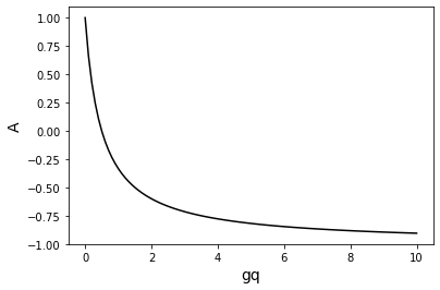
A = \frac{ 1 - 2 \: \gamma q} { 1 + 2\gamma q}.
\end{equation*}\]
where \(q\) ranges from \([0, 1]\). \(\gamma q\) is therefore always positive and bounded between \(0 < \gamma q \leq \gamma\). By plotting this we can clearly see that \(A\) will never be larger than 1. At \(\gamma q=0\), \(A=1\) and for \(\gamma q>0\) then \(A < 1\) .